People from many cultures of the world have a concept of an after life or a heaven. Authors, rulers, artists, spiritualists, and ordinary people have struggled to describe it. The Arabic poet Abu Alaa Al Maarri made such an attempt in ‘Message of Forgiveness’¹ and, more famously for the western world, Dante Alighieri tried in his ‘Divine Comedy’². The Mughal emperor who built the Taj Mahal designed it to mirror the description of heaven given in the Koran. For the author of ‘The Apocalypse of Peter’ the description of heaven is that of a beautiful country, brightly lit, and covered with perfect flowers, fruits and spices which strongly perfume the air.³ In Derek Walcott’s epic poem, Omeros⁴, the protagonist Major Plunkett asks the sibyl Ma Kilman to contact his dead wife in a séance and among other things finds out where she is:

Plunkett never thought he would ask the next question.
“Heaven?” He smiled.

“Yes. If heaven is a green place.”

Grounded in the landscape of this world, is it no wonder that few geographers have attempted to map the landscape of heaven. Though according to John Brinckerhoff Jackson, founding editor of Landscape magazine and a well known geographer, human history brought about human geography and the landscape was simply humankind’s “persistent desire to make earth over in the image of some heaven”.⁵

The purpose of this paper is to make such an attempt; to describe the geography of heaven as depicted by the earthly gateway to that celestial realm: the cemetery. Long after they cease to be used, cemeteries are often still amongst the most cared for of human landscapes. Whether by historical preservation societies, volunteers, local government agencies, or individual families that own plots, cemetery grounds continue to be cared for and maintained. Is there a clue to the heavenly geography in the landscape of cemeteries or at least to our human perception of heaven?

The discipline of Perceptual Geography is the study of the mental maps that people make⁶. People’s perception of place is based upon their own personal experience and knowledge of a particular place and the experience and knowledge they gain from other sources. By default this picture is incomplete; hence perceptual rather than objective.

Perceptual Geography began with John K. Wright’s address, “Terrae Incognitae: The Place of the Imagination in Geography”, given to the American Geographical Society in 1947. He defined it as “the study of geographical knowledge from any and all points of view” and as dealing with “the nature and expression of geographical knowledge both past and present”.

It continued with Kevin Lynch⁷, for whom a person’s mental map of a city consisted of five (5) basic elements:

• Paths – channels thru the city such as streets, rivers, railroads, etc
• Edges – perceived breaks or edges to the city that limit movement
• Nodes – points where navigation decisions have to be made
• Districts – areas with a distinct perceived character
• Landmarks – distinctive and recognizable reference points

Many factors preclude an exhaustive survey of cemeteries across the world or thru history, so some concession must be made for the sake of brevity and practicality. The decision was made to limit the scope of the study to the Sacramento region which provides a sufficient number of cases for a preliminary study and would allow for feasible field research if required. Through out this section the example of Bellevue Cemetery is used for illustration but the outlined processes were executed on all cemeteries in the sample.

The website, Topozone, maintained by Maps a la carte inc. provides lists by feature type within county areas. The list provided at the above link is for Cemeteries in Sacramento County of which there were thirty one (31) when this paper was written. Other sources were also researched such as Yellow Pages⁸, the Tombstone Transcription Project⁹, the California Cemetery and Funeral Bureau¹⁰, and the Cemetery and Mortuary Association of California¹¹ but Topozone was chosen for a number of reasons:

• The number of case study cemeteries provided was generally consistent with the other resources checked.
• Elevation and coordinate information was provided for all entries and was in a consistent format. This would prove useful in location the case studies when searching for aerial photographs of the sites.

Aerial photographs provided by Google were printed so that they could be later scanned for image manipulation software and analyzed in ArcMap12. This source of aerial photographs was used because it’s a free source of the material and it allowed for the reference coordinates to be stored with the scanned photographs and yet not interfere with the landscape image by providing the Google maps service with coordinates adjacent to the case study sites. However, there are problems with using this source of imagery; the images differ in historical timeframe, there are differences in the angle at which the images were taken, differing image resolutions, and differences in scale. But for the purposes of this study these issues were considered to be of minimal import. The scanned images were cropped13 to exclude as much detail from outside the cemetery perimeter as possible. Each of the cemeteries was visited and the perimeter walked with a GPS unit14 logging the track. At some locations there were issues encountered in completing this task:

Satellite Image from Google Maps

• Weather interfering with GPS accuracy.
• Cemeteries closing earlier than anticipated.
• Perimeter location was not always well marked.
• Terrain was rough, overgrown, muddy or otherwise difficult to traverse.
• Tree cover along the perimeter interfered with satellite signal and may result in a loss of accuracy.
• Funeral services at the location on the day of the survey.
• Historical cemeteries on private property may need to be dropped from the study unless the permission of the property owner is obtained.

These tracks were transferred from the unit to MapSource Waypoint Manager¹⁵, named to match the identifier given to each cemetery in a base spreadsheet I maintained, and then edited slightly to remove extraneous track information. This track information, along with the base location file and cemetery imagery converted to KML¹⁶ format, was uploaded to Google Earth to compare the track accuracy with information provide by its imagery. This process revealed circumstances under which the perimeter would need to be re-walked because of inaccuracies in the GPS data but the timeframe permitted for the project did not allow for such rework and so allowances would need to be made in the analysis.

Garmin Waypoint Manager Data

Google Earth Image With KML Overlay

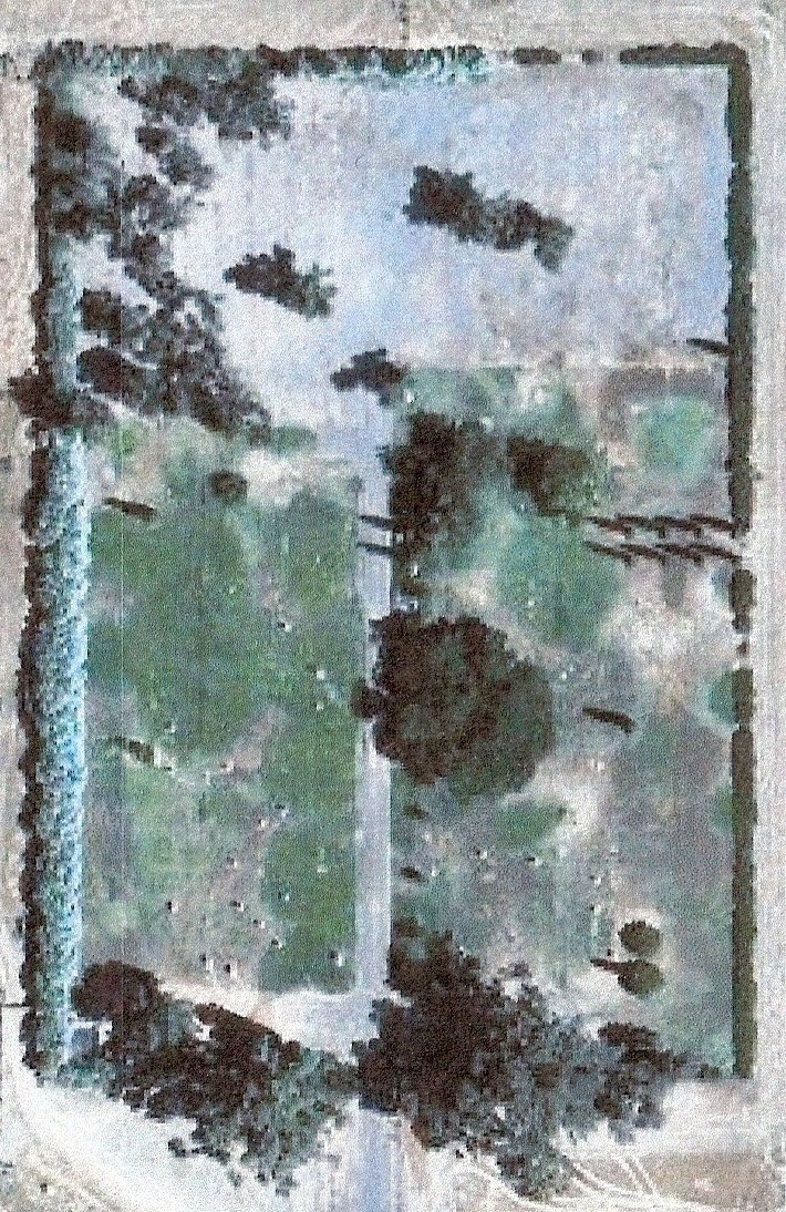
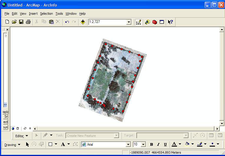
Once the accuracy of the track data was determined the KML files were converted to projected ArcMap point shapefile format using the DNR Garmin Application¹⁷ from the Minnesota Department of Natural Resources. The cropped jpeg image for each cemetery and its associated shapefile was added to ArcMap and the point data from the shapefile mapped to control points on the image so that it could be georeferenced to the GPS track data using the Georeferencing toolbar.

As this proved to be a very time consuming and labor intensive process, the decision as made to limit the study to fourteen (14) cemetery sites within the study area. Additionally, it would have been much better to take perhaps 3 or 4 good waypoints to use for georeferencing rather than the track process utilized. Hindsight is 20/20.

Georeferenced Image
Using Control Points from Converted Garmin data

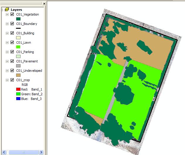
The next step was to create a geodatabase in ArcCatalog for each cemetery, import the related georeferenced raster image, and create a feature dataset containing a standard set of feature classes for each. The first issue was in determining what feature classes to create that would accurately reflect the landscape of the cemetery sample. Where a particular cemetery did not contain a particular feature the associated feature class was still created as a null dataset. The following feature classes were defined as standard:

• Vegetation - a polygon feature class for the areas of tree cover and shrubbery in the cemetery
• Boundary - a polyline feature class to indicate the cemetery boundary
• Building - a polygon feature class for significant structures in the cemetery
• Lawn - a polgon feature class for the manicured sections of the cemetery
• Parking - a polygon feature class for parking areas in the cemetery
• Pavement - a polygon feature class for major roads and pathways thru the cemetery
• Undeveloped - a polygon feature class for the un-manicured and undeveloped area of the cemetery

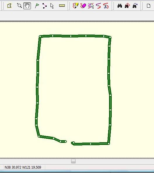
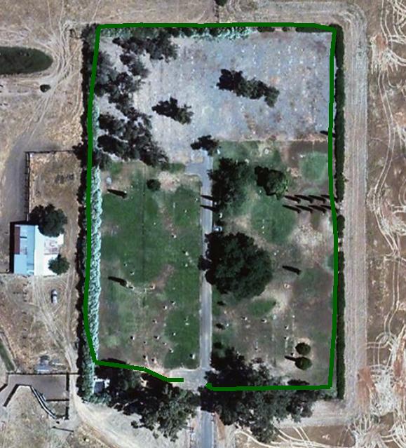
With each database defined, the digitizing process could begin. Care needed to be taken in determining what snapping settings and tolerances were set as some feature classes would overlay each other such as Vegetation with Pavement or Lawn or just about any other feature class. Sometimes the order in which features were digitized, combined with the snapping tolerance set, influenced the size, shape, and area of the digitized feature. There was also the problem of shadow in the source aerial photograph which often made it difficult to determine where vegetation or buildings ended and shadow began. Additionally, and especially with vegetation cover such as tall trees, the problem of radial displacement was significant. Finally, at certain resolutions or zoom levels, features such as buildings, vegetation, and pathways were difficult to digitize or even to determine what the feature was unless a further field trip was organized to gather more data. A compromise needed to be struck for these problems. At all times the original printed image from Google was kept handy for reference purposes. Inevitably, however, the problem of slivers, under or over shoots, and dangling nodes remained and needed to be edited out where necessary to not compromise the final analysis.

Digitized Raster Image
Depicting Defined Feature Classes

Having built the GIS as described, the next step was to analyze the data captured. The simplest analysis to produce was a determination of what percentage of each cemetery's area is taken up by the features digitized. ArcMap's Statistics function provided most of these figures though some Excel massaging did take place. The table below lists the cemeteries in the sample with the percentage of the cemetery area represented by each feature. Note that the percentages do not total 100 since both Vegetation and Buildings overlap the other features in many instances. The cemeteries most closely matching the median and mean values are highlighted as these represent the closest to the ideal as defined by the sample set.

In the chart to the left, the mean of the non overlapping features of the idealized heavenly landscape are depicted.

Though there is ample room for growth, the predominant ground coverage is the Lawn feature.

Pavement and Parking comprise the rest.

In the chart to the left, the median of the non overlapping features of the idealized heavenly landscape are depicted.

Though the Lawn feature comprises a similar proportion to the mean, Pavement takes up a larger portion and Undeveloped a smaller.

Parking comprises a similar portion.

In the chart to the left, the mean of the overlapping features of the idealized heavenly landscape are depicted.

Vegetation comprises a significant proportion of the heavenly landscape with Buildings being a minor element.

In the chart to the left, the median of the overlapping features of the idealized heavenly landscape are depicted.

Vegetation comprises a significant though lesser proportion than at the mean.

Obviously the small data sample greatly affected the outcome of this analysis and the addition of further samples would lead to a different result. Similarly, classifying the cemeteries by historical founding and treating those from similar periods might produce an analysis of the changing perceptions of heaven over the centuries.

The result could be further refined by the introduction and analysis of additional attributes for the classified features. Building could be classified by type - maintenance, mausoleum, or visitor center - or by location - along the cemetery border, in a lawned or undeveloped area. Similarly, vegetation could be further refined by type - tree, hedge, or shrub - or by location since vegetation in undeveloped areas might radically alter once those locations are developed.

Additional concepts not considered in this analysis could also round out the perception of heaven. Elevation and slope were not considered here and might offer some perspective on the heavenly landscape. Population density, growth and development over time, and even degrees of societal stratification might be analyzed by paying closer attention to headstones, graveside borders and adornments.

Lastly, the addition of a new feature class, entrance, with associated attributes such as size, proximity to administrative or visitor center buildings, gated versus open, and many more such attributes could be considered an indication of a societies belief in and respect for the many paths to heaven.

To a degree this is obviously tongue-in-cheek, but everyone who believes in an afterlife probably already has a perception as to what that afterlife looks like. The question this paper tries to answer is the degree to which that perception might be reflected in the cemetery landscape.

¹ al-Iskandarani Mohammad (editor), Risalat Al Ghufran. Dar al-Kitab al-Arabi-Libanon.
² Ciardi John (translator), The Divine Comedy. New York: New American Library, 2003.
³ Adamik Tamas, The Description of Paradise in the Apocalypse of Peter. Leuven, Belgium: Peeters Publishers, 2003.
⁴ Walcott Derek, Omeros. New York: Noonday-Farrar, Straus and Giroux, 1990.
⁵ Baker Alan R.H., Geography and History: Bridging the Divide. Cambridge : Cambridge University Press, 2003.
⁶ Downs Roger M & Meyer James T., Geography and the Mind: An Exploration of Perceptual Geography in American Behavioral Scientist 22 (1978), pp. 59-77 .
⁷ Lynch Kevin, The Image of the City. Cambridge : Cambridge MIT Press, 1960.
⁸ Yellow Pages provided a list of 35 cemeteries in the study area but lacked the elevation and coordinate information of Topozone.
⁹ The Tombstone Transcription Project provided a list of 29 cemeteries in the study area but lacked the elevation and coordinate information of Topozone. It also suffers from being a volunteer site and is therefore not consistent in the data in provides on each cemetery though this is a plus in that many entries come with photographs of the locations.
¹⁰ The California Cemetery and Funeral Bureau did not provide a case study list but was a useful starting point for other related resources.
¹¹ The Cemetery and Mortuary Association of California provided a list of 8 cemeteries in the study area limited to their current membership and lacking the elevation and coordinate information of Topozone.
¹² ArcMap – details of the application can be found at the ESRI website.
¹³ Windows Picture Manager was used to complete the cropping process.
¹⁴ The unit used was a Garmin eTrex Summit HC and specifications can be found at Garmin.
¹⁵ MapSource – details of the application can be found at the Garmin website.
¹⁶ KML is an xml-based language for managing three dimensional geospatial data in Google Earth and Google Maps.
¹⁷ DNR Garmin Application provides the ability to transfer data between a Garmin GPS and various GIS applications including ArcMap from ESRI.

Supporing ArcMap files in a Zip folder